Boston Housing

rpi.analyticsdojo.com

#This uses the same mechansims. 
%matplotlib inline

35. Boston Housing#

Getting the Data
Reviewing Data
Modeling
Model Evaluation
Using Model
Storing Model

35.1. Getting Data#

Available in the sklearn package as a Bunch object (dictionary).
From FAQ: “Don’t make a bunch object! They are not part of the scikit-learn API. Bunch objects are just a way to package some numpy arrays. As a scikit-learn user you only ever need numpy arrays to feed your model with data.”
Available in the UCI data repository.
Better to convert to Pandas dataframe.

#From sklearn tutorial.
from sklearn.datasets import load_boston
boston = load_boston()
print( "Type of boston dataset:", type(boston))

Type of boston dataset: <class 'sklearn.utils.Bunch'>

#A bunch is you remember is a dictionary based dataset.  Dictionaries are addressed by keys. 
#Let's look at the keys. 
print(boston.keys())

dict_keys(['data', 'target', 'feature_names', 'DESCR', 'filename'])

#DESCR sounds like it could be useful. Let's print the description.
print(boston['DESCR'])

.. _boston_dataset:

Boston house prices dataset
---------------------------

**Data Set Characteristics:**  

    :Number of Instances: 506 

    :Number of Attributes: 13 numeric/categorical predictive. Median Value (attribute 14) is usually the target.

    :Attribute Information (in order):
        - CRIM     per capita crime rate by town
        - ZN       proportion of residential land zoned for lots over 25,000 sq.ft.
        - INDUS    proportion of non-retail business acres per town
        - CHAS     Charles River dummy variable (= 1 if tract bounds river; 0 otherwise)
        - NOX      nitric oxides concentration (parts per 10 million)
        - RM       average number of rooms per dwelling
        - AGE      proportion of owner-occupied units built prior to 1940
        - DIS      weighted distances to five Boston employment centres
        - RAD      index of accessibility to radial highways
        - TAX      full-value property-tax rate per $10,000
        - PTRATIO  pupil-teacher ratio by town
        - B        1000(Bk - 0.63)^2 where Bk is the proportion of blacks by town
        - LSTAT    % lower status of the population
        - MEDV     Median value of owner-occupied homes in $1000's

    :Missing Attribute Values: None

    :Creator: Harrison, D. and Rubinfeld, D.L.

This is a copy of UCI ML housing dataset.
https://archive.ics.uci.edu/ml/machine-learning-databases/housing/


This dataset was taken from the StatLib library which is maintained at Carnegie Mellon University.

The Boston house-price data of Harrison, D. and Rubinfeld, D.L. 'Hedonic
prices and the demand for clean air', J. Environ. Economics & Management,
vol.5, 81-102, 1978.   Used in Belsley, Kuh & Welsch, 'Regression diagnostics
...', Wiley, 1980.   N.B. Various transformations are used in the table on
pages 244-261 of the latter.

The Boston house-price data has been used in many machine learning papers that address regression
problems.   
     
.. topic:: References

   - Belsley, Kuh & Welsch, 'Regression diagnostics: Identifying Influential Data and Sources of Collinearity', Wiley, 1980. 244-261.
   - Quinlan,R. (1993). Combining Instance-Based and Model-Based Learning. In Proceedings on the Tenth International Conference of Machine Learning, 236-243, University of Massachusetts, Amherst. Morgan Kaufmann.

# Let's change the data to a Panda's Dataframe
import pandas as pd
boston_df = pd.DataFrame(boston['data'] )
boston_df.head()

	0	1	2	4	5	6	7	8	9	10	11	12
0	0.00632	18.0	2.31	0.538	6.575	65.2	4.0900	1.0	296.0	15.3	396.90	4.98
1	0.02731	0.0	7.07	0.469	6.421	78.9	4.9671	2.0	242.0	17.8	396.90	9.14
2	0.02729	0.0	7.07	0.469	7.185	61.1	4.9671	2.0	242.0	17.8	392.83	4.03
3	0.03237	0.0	2.18	0.458	6.998	45.8	6.0622	3.0	222.0	18.7	394.63	2.94
4	0.06905	0.0	2.18	0.458	7.147	54.2	6.0622	3.0	222.0	18.7	396.90	5.33

#Now add the column names.
boston_df.columns = boston['feature_names']
boston_df.head()

	CRIM	ZN	INDUS	NOX	RM	AGE	DIS	RAD	TAX	PTRATIO	B	LSTAT
0	0.00632	18.0	2.31	0.538	6.575	65.2	4.0900	1.0	296.0	15.3	396.90	4.98
1	0.02731	0.0	7.07	0.469	6.421	78.9	4.9671	2.0	242.0	17.8	396.90	9.14
2	0.02729	0.0	7.07	0.469	7.185	61.1	4.9671	2.0	242.0	17.8	392.83	4.03
3	0.03237	0.0	2.18	0.458	6.998	45.8	6.0622	3.0	222.0	18.7	394.63	2.94
4	0.06905	0.0	2.18	0.458	7.147	54.2	6.0622	3.0	222.0	18.7	396.90	5.33

#Add the target as PRICE. 
boston_df['PRICE']= boston['target']
boston_df.head()

	CRIM	ZN	INDUS	NOX	RM	AGE	DIS	RAD	TAX	PTRATIO	B	LSTAT	PRICE
0	0.00632	18.0	2.31	0.538	6.575	65.2	4.0900	1.0	296.0	15.3	396.90	4.98	24.0
1	0.02731	0.0	7.07	0.469	6.421	78.9	4.9671	2.0	242.0	17.8	396.90	9.14	21.6
2	0.02729	0.0	7.07	0.469	7.185	61.1	4.9671	2.0	242.0	17.8	392.83	4.03	34.7
3	0.03237	0.0	2.18	0.458	6.998	45.8	6.0622	3.0	222.0	18.7	394.63	2.94	33.4
4	0.06905	0.0	2.18	0.458	7.147	54.2	6.0622	3.0	222.0	18.7	396.90	5.33	36.2

35.2. Attribute Information (in order):#

Looks like they are all continuous IV and continuous DV. - CRIM per capita crime rate by town - ZN proportion of residential land zoned for lots over 25,000 sq.ft. - INDUS proportion of non-retail business acres per town - CHAS Charles River dummy variable (= 1 if tract bounds river; 0 otherwise) - NOX nitric oxides concentration (parts per 10 million) - RM average number of rooms per dwelling - AGE proportion of owner-occupied units built prior to 1940 - DIS weighted distances to five Boston employment centres - RAD index of accessibility to radial highways - TAX full-value property-tax rate per 10,000 - PTRATIO pupil-teacher ratio by town - B 1000(Bk - 0.63)^2 where Bk is the proportion of blacks by town - LSTAT % lower status of the population - MEDV Median value of owner-occupied homes in 1000’s Let’s check for missing values.

import numpy as np
#check for missing values
print(np.sum(np.isnan(boston_df)))

CRIM       0
ZN         0
INDUS      0
CHAS       0
NOX        0
RM         0
AGE        0
DIS        0
RAD        0
TAX        0
PTRATIO    0
B          0
LSTAT      0
PRICE      0
dtype: int64

35.3. What type of data are there?#

First let’s focus on the dependent variable, as the nature of the DV is critical to selection of model.
Median value of owner-occupied homes in $1000’s is the Dependent Variable (continuous variable).
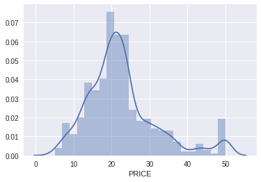
It is relevant to look at the distribution of the dependent variable, so let’s do that first.
Here there is a normal distribution for the most part, with some at the top end of the distribution we could explore later.

#Let's us seaborn, because it is pretty. ;) 
#See more here. http://seaborn.pydata.org/tutorial/distributions.html
import seaborn as sns
sns.distplot(boston_df['PRICE']);

/usr/local/lib/python3.6/dist-packages/matplotlib/axes/_axes.py:6521: MatplotlibDeprecationWarning: 
The 'normed' kwarg was deprecated in Matplotlib 2.1 and will be removed in 3.1. Use 'density' instead.
  alternative="'density'", removal="3.1")

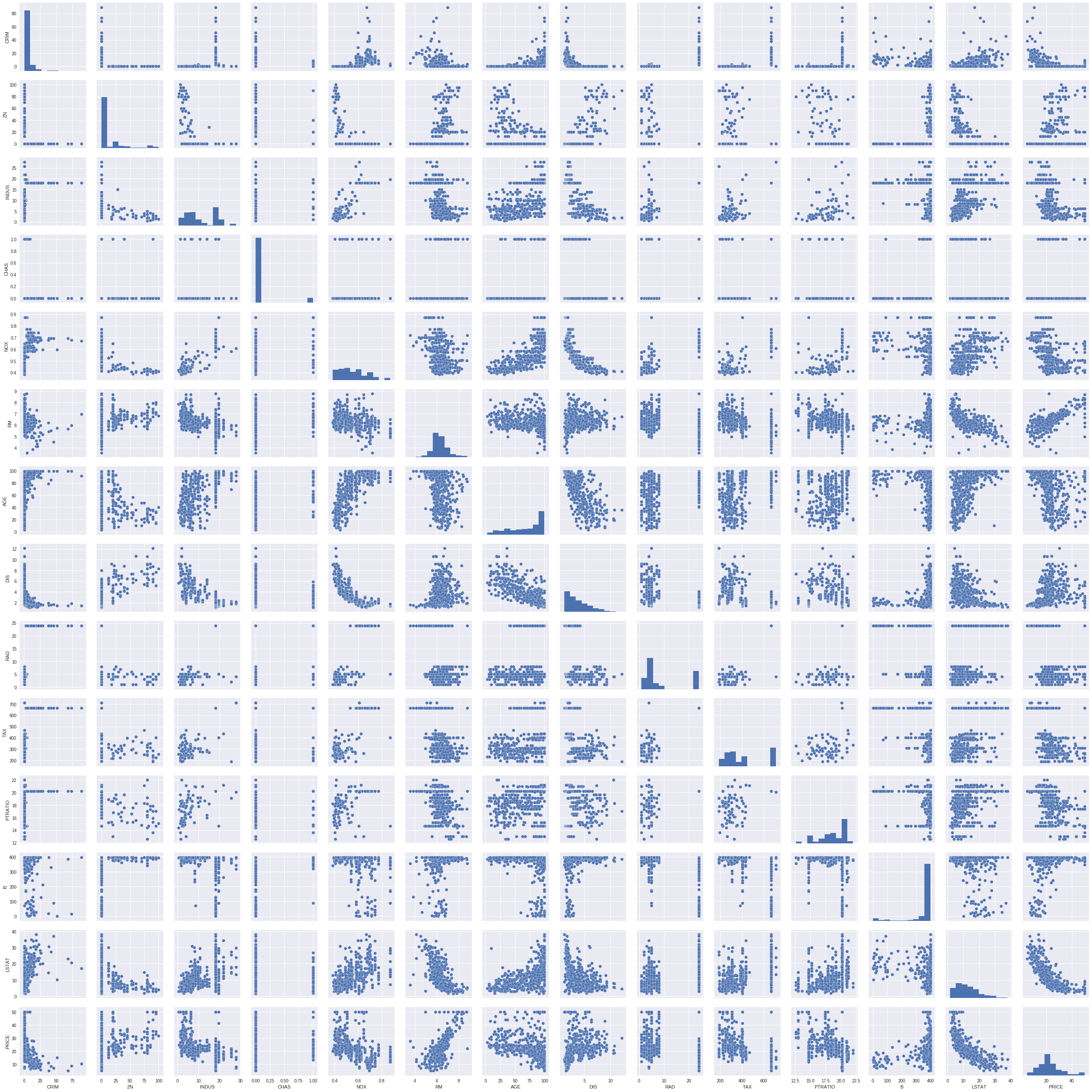
../_images/8bc2de2a37c1cdf1d4b0329eb920f6fb92a2d8612f329c23277538057eb7962e.png

#We can quickly look at other data. 
#Look at the bottom row to see thinks likely coorelated with price. 
#Look along the diagonal to see histograms of each. 
sns.pairplot(boston_df);

../_images/f1dedfef420809550862e77a018219ae5b2186e77481e1b319cb0777896181fc.png

35.4. Preparing to Model#

It is common to separate y as the dependent variable and X as the matrix of independent variables.
Here we are using train_test_split to split the test and train.
This creates 4 subsets, with IV and DV separted: X_train, X_test, y_train, y_test

#This will throw and error at import if haven't upgraded. 
# from sklearn.cross_validation  import train_test_split  
from sklearn.model_selection  import train_test_split
#y is the dependent variable.
y = boston_df['PRICE']
#As we know, iloc is used to slice the array by index number. Here this is the matrix of 
#independent variables.
X = boston_df.iloc[:,0:13]

# Split the data into a training set and a test set
X_train, X_test, y_train, y_test = train_test_split(X, y, test_size=0.3, random_state=0)

print(X_train.shape, X_test.shape, y_train.shape, y_test.shape)

(354, 13) (152, 13) (354,) (152,)

35.5. Modeling#

First import the package: from sklearn.linear_model import LinearRegression
Then create the model object.
Then fit the data.
This creates a trained model (an object) of class regression.
The variety of methods and attributes available for regression are shown here.

from sklearn.linear_model import LinearRegression
lm = LinearRegression()
lm.fit( X_train, y_train )

LinearRegression(copy_X=True, fit_intercept=True, n_jobs=None,
         normalize=False)

35.6. Evaluating the Model Results#

You have fit a model.
You can now store this model, save the object to disk, or evaluate it with different outcomes.
Trained regression objects have coefficients (coef_) and intercepts (intercept_) as attributes.
R-Squared is determined from the score method of the regression object.
For Regression, we are going to use the coefficient of determination as our way of evaluating the results, also referred to as R-Squared

print('labels\n',X.columns)
print('Coefficients: \n', lm.coef_)
print('Intercept: \n', lm.intercept_)
print('R2 for Train)', lm.score( X_train, y_train ))
print('R2 for Test (cross validation)', lm.score(X_test, y_test))

labels
 Index(['CRIM', 'ZN', 'INDUS', 'CHAS', 'NOX', 'RM', 'AGE', 'DIS', 'RAD', 'TAX',
       'PTRATIO', 'B', 'LSTAT'],
      dtype='object')
Coefficients: 
 [-1.21310401e-01  4.44664254e-02  1.13416945e-02  2.51124642e+00
 -1.62312529e+01  3.85906801e+00 -9.98516565e-03 -1.50026956e+00
  2.42143466e-01 -1.10716124e-02 -1.01775264e+00  6.81446545e-03
 -4.86738066e-01]
Intercept: 
 37.937107741833294
R2 for Train) 0.7645451026942549
R2 for Test (cross validation) 0.6733825506400183

#Alternately, we can show the results in a dataframe using the zip command.
pd.DataFrame( list(zip(X.columns, lm.coef_)),
            columns=['features', 'estimatedCoeffs'])

	features	estimatedCoeffs
0	CRIM	-0.121310
1	ZN	0.044466
2	INDUS	0.011342
3	CHAS	2.511246
4	NOX	-16.231253
5	RM	3.859068
6	AGE	-0.009985
7	DIS	-1.500270
8	RAD	0.242143
9	TAX	-0.011072
10	PTRATIO	-1.017753
11	B	0.006814
12	LSTAT	-0.486738

35.7. Cross Validation and Hyperparameter Tuning#

The basic way of having a train and a test set can result in overfitting if there are parameters within the model that are being optimized. Further described here.
Because of this, a third validation set can be partitioned, but at times there isn’t enough data.
So Cross validation can split the data into (cv) different datasets and check results.
Returning MSE rather than R2.

from sklearn.model_selection import cross_val_score
scores = cross_val_score(lm, X_train, y_train, cv=8) 
print("R2:", scores, "\n R2_avg: %0.2f (+/- %0.2f)" % (scores.mean(), scores.std() * 2))

R2: [0.69809776 0.6848557  0.61677678 0.74414545 0.75431003 0.62128711
 0.84406153 0.78197333] 
 R2_avg: 0.72 (+/- 0.15)

35.8. Calculation of Null Model#

We also want to compare a null model (baseline model) with our result.
To do this, we have to generate an array of equal size to the train and test set.

#Here we need to constructor our Base model 
#This syntax multiplies a list by a number, genarating a list of length equal to that number.
#Then we can cast it as a Pandas series.
y_train_base = pd.Series([np.mean(y_train)] * y_train.size)
y_test_base = pd.Series([np.mean(y_train)] * y_test.size)
print(y_train_base.head(), '\n Size:', y_train_base.size)
print(y_test_base.head(), '\n Size:', y_test_base.size)

  22.74548
  22.74548
  22.74548
  22.74548
  22.74548
dtype: float64 
 Size: 354
  22.74548
  22.74548
  22.74548
  22.74548
  22.74548
dtype: float64 
 Size: 152

35.9. Scoring of Null Model#

While previously we generated the R2 score from the fit method, passing X and Y, we can also score the r2 using the r2_score method, which is imported from sklearn.metrix.
The r2_score method accepts that true value and the predicted value.

from sklearn.metrics import r2_score
r2_train_base= r2_score(y_train, y_train_base)
r2_train_reg = r2_score(y_train, lm.predict(X_train))

r2_test_base = r2_score(y_test, y_test_base)
r2_test_reg = r2_score(y_test, lm.predict(X_test))
print(r2_train_base, r2_train_reg,r2_test_base,r2_test_reg  )

-2.220446049250313e-16 0.7645451026942549 -0.006019731947687124 0.6733825506400184

35.10. Scoring of Null Model#

We got a 0 R-squared for our model. Why 0?
This is where it is important to understand what R-squared is actually measuring.
On the left side you see the total sum of squared values (ss_tot_train below).
On the right you see the sum of squares regression (ss_reg_train).
For the null model, the ss_tot_train = ss_reg_train, so R-squared = 0.
By Orzetto (Own work) [CC BY-SA 3.0 (http://creativecommons.org/licenses/by-sa/3.0) or GFDL (http://www.gnu.org/copyleft/fdl.html)], via Wikimedia Commons

#total sum of squares 
ss_tot_train=np.sum((y_train-np.mean(y_train))**2)
ss_res_train=np.sum((y_train-lm.predict(X_train))**2)
ss_reg_train=np.sum((lm.predict(X_train)-np.mean(y_train))**2)

r2_train_reg_manual= 1-(ss_res_train/ss_tot_train)

print(r2_train_reg, r2_train_reg_manual, ss_tot_train, ss_res_train, ss_reg_train )

0.7645451026942549 0.7645451026942549 30006.637768361583 7065.209814240268 22941.427954121522

35.11. Predict Outcomes#

The regression predict uses the trained coefficients and accepts input.
Here, by passing the origional from boston_df, we can create a new column for the predicted value.

boston_df['PRICE_REG']=lm.predict(boston_df.iloc[:,0:13])
boston_df[['PRICE', 'PRICE_REG']].head()

	PRICE	PRICE_REG
0	24.0	30.290795
1	21.6	24.885615
2	34.7	30.471178
3	33.4	28.472236
4	36.2	27.811077

35.12. Graph Outcomes#

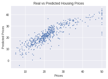
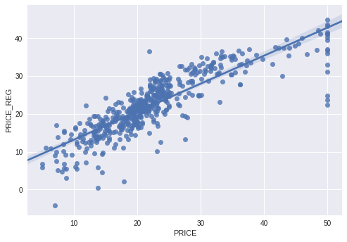
Common to grapy predicted vs actual.
Results should show a randomly distributed error function.
Note that there seem to be much larger errors on right side of grant, suggesting something else might be impacting highest values.

import matplotlib.pyplot as plt
%matplotlib inline
plt.scatter( boston_df['PRICE'], boston_df['PRICE_REG'], s=5 )
plt.xlabel( "Prices")
plt.ylabel( "Predicted Prices")
plt.title( "Real vs Predicted Housing Prices")

Text(0.5, 1.0, 'Real vs Predicted Housing Prices')

../_images/689736fc91bf892b486b16ca64250dd06dc3d8e746f287d40ab3b869c455508e.png

#Let's make it look pretty with pickle
import seaborn as sns; sns.set(color_codes=True)
ax = sns.regplot(x="PRICE", y="PRICE_REG", data=boston_df[['PRICE','PRICE_REG']])

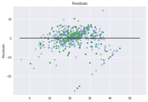
../_images/0305b43f78b387f688375c66cbcb481d39afd685ba3c381982a0966a06215e37.png

35.13. Graph Residuals#

Common to graph predicted - actual (error term).
Results should show a randomly distributed error function.
Here we are showing train and test as different

#
plt.scatter( lm.predict(X_train), lm.predict(X_train) - y_train,
           c ='b', s=30, alpha=0.4 )
plt.scatter( lm.predict(X_test), lm.predict(X_test) - y_test,
           c ='g', s=30 )
#The expected error is 0. 
plt.hlines( y=0, xmin=-5, xmax=55)
plt.title( "Residuals" )
plt.ylabel( "Residuals" )

Text(0, 0.5, 'Residuals')

../_images/9ba6de96d3f256197632f9f5518b597dbb3991a66316c02bfb10d4590746c412.png

35.14. Persistent Models#

I could be that you would want to maintain
The pickle package enables storing objects to disk and then retreive them.
For example, for a trained model we might want to store it, and then use it to score additional data.

#save the data
boston_df.to_csv('boston.csv')

import pickle
pickle.dump( lm, open( 'lm_reg_boston.p', 'wb' ) )

#Load the pickled object. 
lm_pickled = pickle.load( open( "lm_reg_boston.p", "rb" ) )

lm_pickled.score(X_train, y_train)

0.7645451026942549

Copyright AnalyticsDojo 2016. This work is licensed under the Creative Commons Attribution 4.0 International license agreement.

Boston Housing

Contents

Boston Housing

rpi.analyticsdojo.com

35. Boston Housing#

35.1. Getting Data#

35.2. Attribute Information (in order):#

35.3. What type of data are there?#

35.4. Preparing to Model#

35.5. Modeling#

35.6. Evaluating the Model Results#

35.7. Cross Validation and Hyperparameter Tuning#

35.8. Calculation of Null Model#

35.9. Scoring of Null Model#

35.10. Scoring of Null Model#

35.11. Predict Outcomes#

35.12. Graph Outcomes#

35.13. Graph Residuals#

35.14. Persistent Models#